AI For Humanity

Lecture 2 - Tree-based methods and Neural Networks

Jonas Skjold Raaschou-Pedersen

2025-09-10

Tree-based Methods

• Why Tree-based methods?
  • Performs well on tabular data
  • Decision Trees, Random Forest, XGBoost are tree-based methods
  • Hence good to know the fundamentals!
  • Naturally handle mixed feature types (numeric & categorical)
  • Provide interpretability (e.g. decision tree diagrams)
  • Require minimal preprocessing (no scaling needed, robust to outliers)
• Later on in the course we consider the Causal Forest method
  • Builds upon Random Forests
• And so we build the foundation

Setup

Consider a dataset with outcomes belonging to \(3\) classes…

Setup

The Iris dataset (Fisher, 1936)

Setup

from sklearn.datasets import load_iris

print(load_iris().DESCR)

yields:

:Number of Instances: 150 (50 in each of three classes)
:Number of Attributes: 4 numeric, predictive attributes and the class
:Attribute Information:
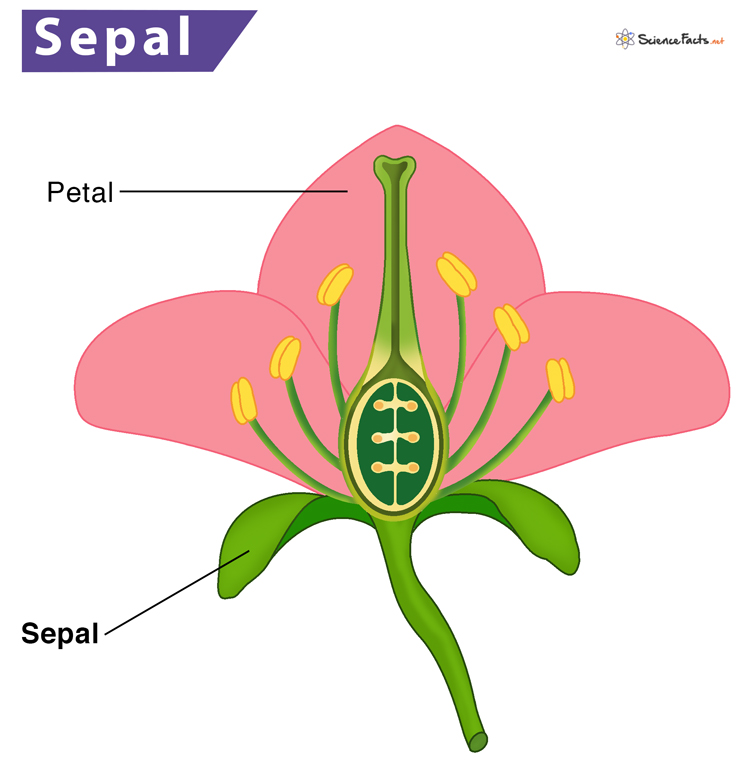
    - sepal length in cm
    - sepal width in cm
    - petal length in cm
    - petal width in cm
    - class:
            - Iris-Setosa
            - Iris-Versicolour
            - Iris-Virginica

============== ==== ==== ======= ===== ====================
                Min  Max   Mean    SD   Class Correlation
============== ==== ==== ======= ===== ====================
sepal length:   4.3  7.9   5.84   0.83    0.7826
sepal width:    2.0  4.4   3.05   0.43   -0.4194
petal length:   1.0  6.9   3.76   1.76    0.9490  (high!)
petal width:    0.1  2.5   1.20   0.76    0.9565  (high!)
============== ==== ==== ======= ===== ====================

• Goal: classify iris flowers to the three categories
• Approach: we’ll use a Decision Tree as our classifier

source 1 & 2

All 2-combinations of features

Could we carve out the feature space…?

Asking questions to the data

Questions that arise

• How do “ask questions to the data” i.e. how do we choose a split?
• How do we measure how “good” a split is?
• When to stop splitting?
• How to make predictions in the leaves?

Approach we’ll take

• Cannot consider every possible partition of the feature space into e.g. \(J\) boxes
• Instead: top-down, greedy approach known as recursive binary splitting
  • top-down: starts at top of tree then successively splits data (indicated via branches)
  • greedy: at each step, the best split is locally optimal (doesn’t look ahead)
  • recursive: after splitting, solve similar problem on the two subsamples
  • binary: the splits are binary (yielding a binary tree; see previous slide)

Setup

• Data tuple \((X, Y) \in \mathcal{X} \times \mathcal{Y}\) where \(\mathcal{X}\) is the feature space and \(\mathcal{Y}\) the outcome space
  • Classification: \(\mathcal{Y} = \{1, 2, \ldots, K\}\)
  • Regression: \(\mathcal{Y} = \mathbb{R}\)
    • Note: we won’t consider Regression Trees in the lecture; only in the exercise class
  • Iris data:
    • \(\mathcal{X} = \mathbb{R}^{4}\) (sepal length, sepal width, petal length, petal width)
    • \(\mathcal{Y} = \{1, 2, 3\}\) (Setosa, Versicolour, Virginica)
• Dataset \(\{(X_{i}, Y_{i})\}_{i=1}^{n}\) (e.g. \(n = 150\) in the Iris data)
• ESLII and ISL books both denote nodes in the decision tree as “boxes”; I’ll instead follow the notation and terminology in (Breiman, 1984)
• Node: A node \(t\) is defined as a subset of \(\mathcal{X}\) (the feature space) i.e. \(t \subset \mathcal{X}\)
  • Example: \(t = \{X_{i} \mid X_{i, 3} \leq 2.45\}\) (all samples with petal length \(\leq\) 2.45 cm)
• Nonterminal node: a node where a split is made
• Terminal node: a node where no further split is made

Inspecting the Tree

• Question: consider \(X_{i} = (6.1, 2.6, 5.6, 1.4)^{T}\); what is the predicted label \(\hat{Y}_{i}?\)
  • Order of \(X\) variables: (sepal length, sepal width, petal length, petal width)

Construction of tree

• Construction of a tree:
  1. Selecting the splits
  2. Declaring a node terminal or continue splitting it
  3. Assignment of each terminal node to a class
• Class assignment is simple
• Main problem: finding good splits and knowing when to stop splitting
• We want to the split of each node so that the data in each of the descendant nodes are “purer” than the data in the parent node

Counting and proportions

• Define:
  • \(N\): total number of samples
  • \(N_{j}\): total number of samples in class \(j\)
  • \(N(t)\): number of samples going to node \(t\)
  • \(N_{j}(t)\): number of samples going to node \(t\) of class \(j\)
• Let \(p(t)\) be the proportion of samples going to node \(t\); \(p(j, t)\) the proportion going to node \(t\) and being class \(j\); and \(p(j \mid t)\) the proportion being class \(j\) given node \(t\)
• Then we can compute the proportions: \[\begin{aligned} &p(t) = \frac{N(t)}{N} \\ &p(j, t) = \frac{N_{j}(t)}{N} \\ &p(j \mid t) = p(j, t) / p(t) = \frac{N_{j}(t)}{N} / \frac{N(t)}{N} = \frac{N_{j}(t)}{N(t)} \end{aligned}\]

Counting and proportions

• Consider the split of node \(t\) into \(t_{L}\) and \(t_{R}\) (left and right), then the following holds: \[\begin{aligned} & p(t_{L}) + p(t_{R}) = p(t) \\ & p_{L} = \frac{p(t_{L})}{p(t)}, \ p_{R} = \frac{p(t_{R})}{p(t)}, \ p_{L} + p_{R} = 1 \end{aligned}\] where \(p_{L}\) is the proportion going to the left node and \(p_{R}\) to the right

• E.g. cf. previous slide \[\begin{aligned} p_{L} = \frac{p(t_{L})}{p(t)} = \frac{ \frac{N(t_{L})}{N} }{ \frac{N(t)}{N} } = \frac{N(t_{L})}{N(t)} \end{aligned}\]

Inspecting the Tree

• Question: consider the nonterminal node with \(N(t) = 84\).

  • Compute the vector of estimated conditional probabilities: \[ (p(1 \mid t), p(2 \mid t), p(3 \mid t))^{T} \] using the expression on the previous slides and the counts in the tree
  • Compute \(p_{L}\) and \(p_{R}\) relative to the same node \(t\)

Approaching a criterion for splitting

• Define impurity measure of node \(t\): \[\begin{aligned} i(t) = \phi(p(1 \mid t), \ldots, p(K \mid t)) \end{aligned}\] where \(\phi\) is the impurity function defined on all \(K\)-tuples of probabilities

• Goodness of split \(s\) for node \(t\): \[\begin{aligned} \Delta i(s, t) & := i(t) - p_{R}i(t_{R}) - p_{L}i(t_{L}) \\ &= i(t) - \frac{N(t_{R})}{N(t)}i(t_{R}) - \frac{N(t_{L})}{N(t)}i(t_{L}) \end{aligned}\]

• The split \(s\) splits node \(t\) into two disjoint subsets \(t_{L}\), \(t_{R}\)

• Splitting rule: at each nonterminal node \(t\) the split selected, \(s^{*}\), is the one which maximizes \(\Delta i(s, t)\) i.e. \(\Delta i(s^{*}, t) = \max_{s} \Delta i(s, t)\)

  • The split should decrease the weighted impurity of nodes \(t_{L}\) and \(t_{R}\) compared to \(t\)

Split \(s\)

Illustration of split from (Breiman, 1984)

Impurity functions

• Gini index: \[\begin{aligned} \phi(p(1 \mid t), \ldots, p(K \mid t)) = \sum_{j = 1}^{K} p(j \mid t)(1 - p(j \mid t)) \end{aligned}\]

• Entropy: \[\begin{aligned} \phi(p(1 \mid t), \ldots, p(K \mid t)) = -\sum_{j = 1}^{K} p(j \mid t) \log p(j \mid t) \end{aligned}\]

• Misclassification error \[\begin{aligned} \phi(p(1 \mid t), \ldots, p(K \mid t)) = 1 - \max_{} p(j \mid t) \end{aligned}\]

• Using the Misclassification error as impurity function has drawbacks

  • The criterion may be zero for all splits \(s\)
  • Isn’t a good criterion for the overall multistep tree growing procedure
  • Reducing the misclassification rate does not appear to be a good criterion

Impurity functions

In the two-class case; image from ESLII.

Computing impurity

• With \(i(t) = \sum_{j = 1}^{K} p(j \mid t)(1 - p(j \mid t))\) (Gini impurity function) and the expression

\[\begin{aligned} \Delta i(s, t) = i(t) - p_{R}i(t_{R}) - p_{L}i(t_{L}) \end{aligned}\]

we can seek the best split \(s\) for each nonterminal node

Computing impurity

• Question: compute \(\Delta i(s, t)\) for the nonterminal node from before with \(N(t) = 84\); you can use the function below and \(p_{L}\) and \(p_{R}\) from before.

def gini_from_counts(N_j_t: np.ndarray, N_t: int):
    p_j_t = N_j_t / N_t
    return float(np.sum(p_j_t * (1 - p_j_t)))

Building a Tree

• With the splitting rule that seeks \(s\) that maximizes \(\Delta i(s, t)\) you are ready to build/grow a tree!
• One stopping rule is to stop growing the tree whenever a split would result in either terminal node having less than min_samples_leaf samples
  • this parameter is found in sklearn as well; they denote terminal nodes by leafs
• We leave out details for how to search for the splits to the exercise class

Growing (our toolbox)

Define:

• Majority label at node \(t\): \(k(t) := \underset{j}{\arg\max} \ p(j \mid t)\)

• Resubstitution estimate \[\begin{aligned} r(t) = 1 - \max_{j}p(j \mid t) = 1 - p(k(t) \mid t) \end{aligned}\]

• Node misclassification cost: \(R(t) := r(t)p(t)\)

• Tree misclassification cost: \[\begin{aligned} R(T) = \sum_{t \in \tilde{T}} R(t) = \sum_{t \in \tilde{T}}r(t)p(t). \end{aligned}\]

where \(\tilde{T}\) is the set of all terminal nodes.

Problem with growing

• Problem: If we split a node \(t\) into child nodes the misclassification rate is ensured to improve; i.e. for any split of a node \(t\) into \(t_{L}\) and \(t_{R}\), \[\begin{aligned} R(t) \geq R(t_{L}) + R(t_{R}). \end{aligned}\]
• The resubstitution error rate is biased downwards; this means that if we simply minimize the resubstitution error rate, we would always prefer a bigger tree.
  • Overfitting!
• Strategy is:
  • Grow a large tree \(T_{max}\) until stopping criteria (e.g. min_samples_leaf) is met
  • prune the tree (i.e. delete nodes) in a clever way

Pruning

• Cost-complexity measure \[\begin{aligned} R_{\alpha}(T) = R(T) + \alpha \vert \tilde{T} \vert \end{aligned}\]
• Can think of \(\alpha\) as the complexity cost per terminal node
  • High \(\alpha\) \(\rightarrow\) simpler tree; low \(\alpha\) \(\rightarrow\) more complex tree
• Finding optimal sequence of \(\alpha\) is called cost-complexity pruning
  • Unfortunately we won’t have time for it
  • See here or here if you are interested [or ch. 3. (Breiman, 1984)]
• Finally, \(K\)-fold cross-validation is used to choose \(\alpha\)

The running example

• See code here

from sklearn.datasets import load_iris
from sklearn.model_selection import train_test_split
from sklearn.tree import DecisionTreeClassifier, plot_tree


X, y = load_iris(return_X_y=True)
X_train, X_test, y_train, y_test = train_test_split(
    X, y, random_state=2025, train_size=0.8
)
clf = DecisionTreeClassifier(
    min_samples_leaf=5,
    criterion="gini",
    random_state=2025,
)
clf.fit(X_train, y_train)

fig, axes = plt.subplots(nrows=1, ncols=1, figsize=(8, 8))
plot_tree(
    clf,
    filled=False,
    proportion=False,
    ax=axes,
    impurity=True,
    feature_names=[
      'sepal length (cm)',
      'sepal width (cm)',
      'petal length (cm)',
      'petal width (cm)'
    ],
)
# plt.savefig("figs/iris_dt2.png", bbox_inches="tight", pad_inches=0)

From Trees to Forests

• Bagging
  • Build many trees on bootstrapped samples
  • Bagged Trees
• Random Forests
  • Build many trees on bootstrapped samples
  • Improvement over Bagged Trees: Random subset of features at each split
  • Decorrelating the trees
  • Aggregate predictions (majority vote / average)
• Boosting
  • Boosting: grow trees sequentially, each focusing on previous errors → reduces bias
• Random Forests are easy to implement once we know Decision Trees / Regression Trees
  • Hence all the time spent on Decision Trees!

Trees and Forests

• Enough with the trees and flowers
  • Although if you haven’t already, go visit Landbohøjskolens Have; 10/10

Neural Networks

• Fundamental method that underlies all of the generative AI revolution
  • Transformers = fancy neural networks
• Large subject: today we’ll focus on a simple example but still with a lot of depth
• In the next lectures you will build upon this e.g. when considering language models

Setup

• The MNIST dataset consists of 70,000 images of handwritten digits (0–9), each a 28 × 28 pixel grayscale image
  • 50,000 training images; 10,000 validation images; 10,000 test images

• We reshape the pixel matrices into \(28 \cdot 28 = 784\)-dimensional vectors, \(x_{i} \in \mathbb{R}^{784 \times 1}\); also, we divide them by \(255\)
• We one-hot encode the labels \(y_{i} \in \{0, 1\}^{10 \times 1}\) (with a \(1\) at the index corresponding to the true label and \(0\) elsewhere)
• Our goal is to estimate a neural network (think of it as a complex non-linear statistical model) to correctly predict the class labels

A Neural Network

source

Neural Network Model

• A neural network takes as input \(x \in \mathbb{R}^{784 \times 1}\) and succesively transforms it as follows. Below we set \(a^{0} = x\)
• Activations of \(j\)th neuron in the \(l\)th layer related to the actions in the \((l - 1)\)th layer by: \[\begin{aligned} a^{l}_{j} = \sigma \left( \sum_{k} w_{jk}^{l} a^{l-1}_{k} + b_{j}^{l} \right) = \sigma (z^{l}_{j}) \end{aligned}\] \[\begin{aligned} z^{l}_{j} = \sum_{k} w_{jk}^{l} a^{l-1}_{k} + b_{j}^{l} \end{aligned}\]
• Weight notation \(w^{l}_{jk}\) to denote weight for the connection from the \(k\)th neuron in the \((l - 1)\)th layer to the \(j\)th neuron in the \(l\)th layer
• \(b_{j}^{l}\) for the \(j\)th bias in the \(l\)th layer

Neural Network Weights

Loss function

• To measure whether our predictions are correct we need a loss function
• Let \(\hat{y} \in \mathbb{R}^{10 \times 1}\) be the predictions from our neural network model based on input \(x\)
  • They are predicted probabilities of being in each of the \(10\) classes
• We will measure how good our model is by the cross-entropy loss function:

\[\ell := \text{CE}(y, \hat{y}) := -\sum_{j=1}^{10} y_j \log \hat{y}_j\]

• For a sample of \(n\) observations the loss is:

\[\mathcal{L} := -\frac{1}{n}\sum_{i=1}^{n}\sum_{j=1}^{10} y_{i, j} \log \hat{y}_{i, j}\]

Loss function - Intuition

Again:

\[\ell = -\sum_{j=1}^{10} y_j \log \hat{y}_j\]

• We want to minimize this function; note:
  • Only one term in the sum is non-zero, the one corresponding to the true label, \(j\), say
  • Also, \(\hat{y}_{j} \in (0, 1)\) so \(\log \hat{y}_{j} \in (-\infty, 0)\) and \(-\log \hat{y}_{j} \in (0, \infty)\)
  • To minimize \(-\log \hat{y}_{j}\) we want \(\hat{y}_{j}\) as close to \(1\) as possible; i.e. we want our model to have as high a predicted probability for the true class as possible

Neural Network Model Vectorized

• Can write the previous equations as vectors: \[\begin{aligned} z^{l} := W^{l}a^{l-1} + b^{l}, \quad a^{l} = \sigma \left(z^{l}\right) \end{aligned}\] where \(W^{l}\) has dimension \(d_{l+1} \times d_{l}\) (dimension of layer \(l + 1\) times that of layer \(l\))
• \(\sigma\) is the sigmoid function for the intermediate layers while it is the softmax function for the output (final) layer
• We denote the softmax function by \(\mathrm{sm}\): \[\begin{aligned} \mathrm{sm}: \mathbb{R}^K \to \mathbb{R}^K,\qquad \mathrm{sm}(z)_i = \frac{\exp (z_{i})}{\sum_{j=1}^K \exp (z_{j})}. \end{aligned}\]
• Transforms a given vector \(z\) into a vector of probabilities
• Very handy when we want to classify digits (or predict the next token in a sentence, to be introduced later in the course)

Neural Network Model - Forward pass

• In the simplest example in Nielsen’s code he uses the following input sizes \((784, 30, 10)\) leading to the weight matrices: \[\begin{aligned} W^{1} \in \mathbb{R}^{30 \times 784}, \ W^{2} \in \mathbb{R}^{10 \times 30}, \ b^{1} \in \mathbb{R}^{30 \times 1}, \ b^{2} \in \mathbb{R}^{10 \times 1}. \end{aligned}\]
• A given input vector \(x \in \mathbb{R}^{784 \times 1}\) (with one-hot encoded label \(y\)) is passed through the network as: \[\begin{aligned} & \mathbb{R}^{30 \times 1} \ni a^{1} = \sigma(z^{1}) = \sigma(W^{1}x + b^{1}) \\ & \mathbb{R}^{10 \times 1} \ni \hat{y} := a^{2} = \mathrm{sm}(z^{2}) = \mathrm{sm}(W^{2}a^{1} + b^{2}) \end{aligned}\] and then compute the loss as: \[\begin{aligned} \ell := \text{CE}(y, \hat{y}) := -\sum_{j=1}^{10} y_j \log \hat{y}_j \end{aligned}\]

Neural Network Model - Code example

• go through function example_lecture in scripts/estimate_network_mn_rw.py until backpropagation part

Updating the parameters

• We update the parameters using stochastic gradient descent (SGD)

• To perform SGD we need to compute the derivatives of the loss function wrt. our parameters: \[ \frac{\partial \ell}{\partial \theta}, \quad \theta = (W^{1}, W^{2}, b^{1}, b^{2}) \]

• Spelling out the loss function for our two-layer network:

\[\begin{aligned} \ell := \text{CE}(y, \hat{y}) := -\sum_{j=1}^{10} y_j \log \hat{y}_j = -\sum_{j=1}^{10} y_j \log \mathrm{sm}(W^{2}\sigma(W^{1}x + b^{1}) + b^{2})_{j} \end{aligned}\]

• Want:

\[ \frac{\partial \ell}{W^{1}}, \ \frac{\partial \ell}{b^{1}}, \ \frac{\partial \ell}{W^{2}}, \ \frac{\partial \ell}{b^{2}} \]

Updating the parameters

• SGD updates as:

\[ \theta \leftarrow \theta - \eta \frac{\partial \ell}{\partial \theta} \] for \(\eta\) the learning rate; step in opposite direction of steepest ascent

• But that doesn’t answer the question of how to compute the derivatives
  • Backpropagation does that!

Backpropagation - Equations

Backpropagation

• Do I have to understand backpropagation?
  • Yes, says Andrey Karpathy (superstar AI researcher)
    • see “Yes you should understand backprop”
    • Broadens your understanding of neural net training
    • Can come in handy when debugging training
    • Good to know in general
    • Demystifies neural nets

Backpropagation - example

• It can be shown that the error of the output layer with the cross-entropy loss function equals: \[\begin{aligned} \delta^{l_{2}} = \frac{\partial \ell}{\partial z^{l_{2}}} = \frac{\partial \ell}{\partial \hat{y}} \frac{\partial \hat{y}}{\partial z^{l_{2}}} = \hat{y} - y. \end{aligned}\]
  • \(\frac{\partial \ell}{\partial \hat{y}}\) the derivative of cross-entropy loss wrt. predicted probabilities
  • \(\frac{\partial \hat{y}}{\partial z^{l_{2}}}\) the derivative of softmax function wrt. input vector
• Then we compute the derivatives: \[\begin{aligned} \frac{\partial \ell}{\partial b^{l_{2}}} = \delta^{l_{2}}, \quad \frac{\partial \ell}{\partial W^{l_{2}}} = \delta^{l_{2}}(a^{l_{1}})^{T} \end{aligned}\]
• Note that \(a^{l_{1}} \in \mathbb{R}^{30 \times 1}\), \(\delta^{l_{2}} \in \mathbb{R}^{10 \times 1}\), and we want to update \(W^{2} \in \mathbb{R}^{10 \times 30}\); hence we should compute the outer product of \(\delta^{l_{2}}\) and \(a^{l_{1}}\) yielding the expression above.

Backpropagation - example continued

• Next, we backpropagate the errors to the first layer: \[\begin{aligned} \delta^{l_{1}} = [(W^{l_{2}})^{T} \delta^{l_{2}}] \odot \sigma'(z^{l_{1}}) = [(W^{l_{2}})^{T} \delta^{l_{2}}] \odot (\sigma(z^{l_{1}}) \odot [\iota - \sigma(z^{l_{1}})]) \end{aligned}\] where \(\iota\) a vector of ones and we used the derivative of the sigmoid function (e.g. equation (4) last week) and then update the weights in the first layer with the derivatives: \[\begin{aligned} \frac{\partial \ell}{\partial b^{l_{1}}} = \delta^{l_{1}}, \quad \frac{\partial \ell}{\partial W^{l_{2}}} = \delta^{l_{1}}(a^{l_{0}})^{T} \end{aligned}\] where we compute the outer product of \(\delta^{l_{2}} \in \mathbb{R}^{30 \times 1}\) and \(a^{l_{0}} \in \mathbb{R}^{784 \times 1}\) to update \(W^{1} \in \mathbb{R}^{30 \times 784}\).

• Update using just computed derivatives and rule \(\theta \leftarrow \theta - \eta \frac{\partial \ell}{\partial \theta}\)

Backpropagation - code example

• go through backprop in function example_lecture in scripts/estimate_network_mn.py
• see code here
• torch example: automatic differentiation
  • scripts/estimate_network_torch.py
  • have to implement yourself at exercise class

Extensions

• Nielsen’s implementation passes single vectors through the network one at a time
  • Inefficient
  • Can pass \((B, 784)\) matrices of batches through the network and backprop at once
• Regularization
  • Dropout
  • Weight decay
• Weight initialization
• More…
• We’ll probably return to it

Wrap up

• Implementation details are left for the exercise classes